1 Intro to R and Co.
In this session you should learn:
1.1 What is R?
From the R project website:

R is a language and environment for statistical computing and graphics.
R provides a wide variety of statistical (linear and nonlinear modelling, classical statistical tests, time-series analysis, classification, clustering, …) and graphical techniques, and is highly extensible.
One of R’s strengths is the ease with which well-designed publication-quality plots can be produced, including mathematical symbols and formulae where needed. Great care has been taken over the defaults for the minor design choices in graphics, but the user retains full control.
R is available as Free Software under the terms of the Free Software Foundation’s GNU General Public License in source code form. It compiles and runs on a wide variety of UNIX platforms and similar systems (including FreeBSD and Linux), Windows and MacOS.
If you are working in your own laptop!
To check if you have R and its version, go to your terminal and type
R --version. If you get an error, you don’t have R installed. If you get a printed output make a note of the version. If it is lower than4, please upgrade. You can download R here.If you are using Windows, you will need RTools, which provides toolchains for building R and R packages from source on Windows. Install it for the corresponding R version you downloaded or have.
Find more info in the complementary course materials (Section 6 of the Syllabus).
1.2 Some quick facts and good-to-know’s
Different to compiled language, like C or JAVA, R’s default implementation is an interpreted language. R is a dynamic programming language, which means R automatically interprets your code as you run it.
R packages are organized via The Comprehensive R Archive Network (CRAN). Mature R packages are submitted to CRAN where checks are performed on their backward compatibility against other packages and R versions and operating systems.
CRAN is a network of ftp and web servers around the world that store identical, up-to-date, versions of code and documentation for R 1.
R uses a particular assign operator:
<-. However, you will see code and in particular in this lessons using:=. You can use them interchangeably and this won’t affect your code. So if you are used to Python, you can stick to=.R has different coding paradigms, most importantly base or vanilla R, tidyverse and data.table.
Piping: if you are familiar with the R tidyverse, you might have seen the use of the
%>%operator to concatenate functions. Since R 4.1.0 R introduced a native pipe operator|>and that is what we use in this course. If you are curious about how the native pipe works and differences with themagrittrpipe, see here and here.
1.3 Why R?

Free and open-source software
Reproducibility
Good package maintenance
Statistical capabilities
Handling geographic and non-geographic data
Visualisation
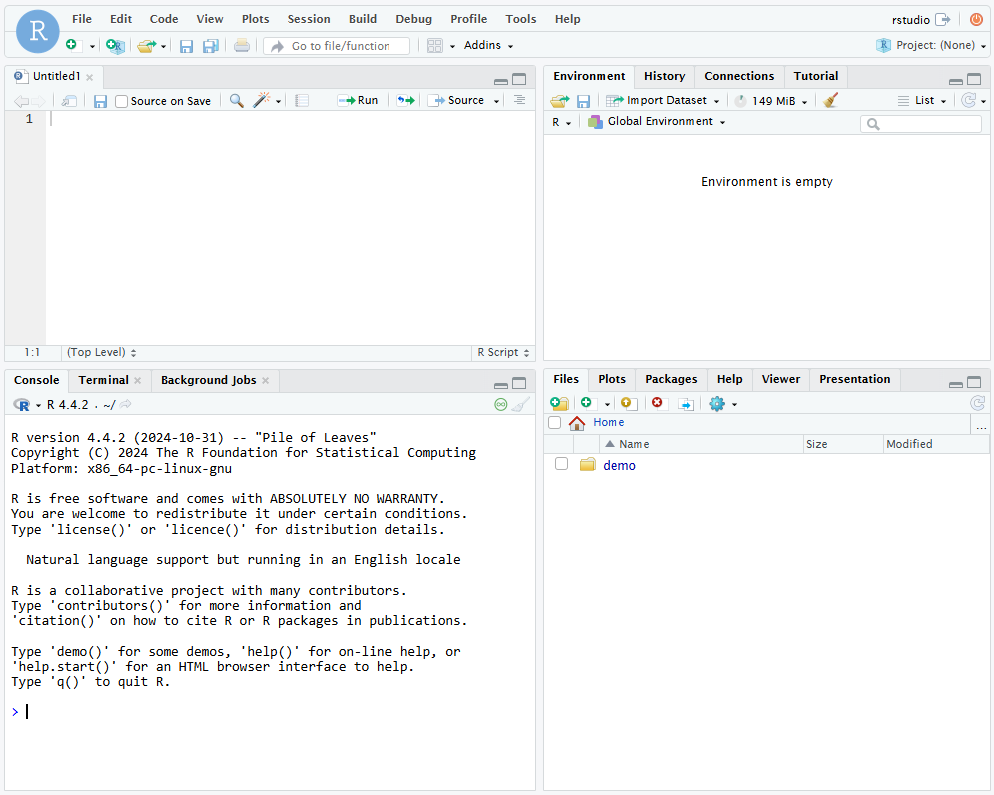
1.4 RStudio
The most well-known IDE to work with R is RStudio, which we will be using throughout this course.
If you are feeling adventurous and would like to be a beta tester of new IDEs, feel free to explore Positron. Beware though, Positron is an early stage project under active development. Get to know if Positron is a good fit for you here.
Disclaimer: I might not be able to help much if you decide to use Positron.
Look for RStudio on your computer, and check its version. To do so, open RStudio, go to Help > About Rstudio. Check your version and that Quarto is also mentioned. You should be having a version higher than RStudio v2022.07, but I recommend to upgrade to the latest version to minimize errors.
Download the latest RStudio version here.
Find more info in the complementary course materials (Section 6 of the Syllabus).
The things that I usually change straight away in Tools > Global Options…
- Strongly recommended:
- In General, make sure that:
- “Restore .RData into workspace ar startup” is unticked
- “Save workspace to .RData on exit” is set to Never
- “Always save history” is unticked
- In Code, tick “Use native pipe operator, |> (requires R 4.1+)”
- In General, make sure that:
- Optional:
- In Appearance, you can change your Editor theme and font size
- In Pane Layout, you can move the panel order. I usually have the console on the top right and the Environment on the bottom left.
1.4.1 RStudio projects
For this course, I would like you to get used to working with projects. Projects are a great way to help you stay organised and have all your scripts, data and output documents and figures in one single place.
You can create a project for this class with the following steps:
- Go to the File > New Project….
- Specify if you would like to create the project in a new directory, or in an existing directory. Select “New Directory”
- RStudio offers dedicated project types if you are working on an R package, or a Shiny Web Application. Here we select “New Project”, which creates an R project
- Give your project a name, something like app_dev_gis and choose the location to save your project
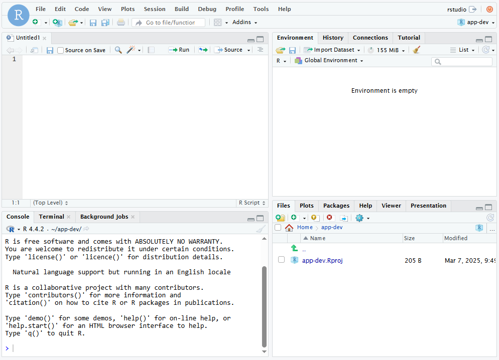
You will see that the project name is in the top-right corner and that there is a .Rproj in the files tab. Any new file you add to the directory will appear here.
I suggest you to use a folder structure that makes sense for your work. In the course, we will have a set of hands-on exercises and practicals, so you can create two sub-directories to store each.
You can also save your final project inside this project if you choose R, however, I suggest you use a completely new project for that, to keep all files separated and a single environment for that.
1.5 Quarto
In this course, we will be using Quarto documents for the practicals. This website itself is created using Quarto.
- Quarto is an open-source scientific and technical publishing system.
- It allows you to combine code, results and text in a single document.
- It uses Markdown syntax.
- With Quarto, you can create reproducible documents in several output formats like PDF, HTML, Word, presentations with Reveal.js, etc.
- It has native support for multiple programming languages like Python and Julia in addition to R.
- It can also render Jupyter notebooks.
1.5.1 Anatomy of a Quarto file
A plain text file that has the extension .qmd is a Quarto file:
---
title: I am a Quarto file
date: today
format: html
---

In this document, we will load a *spatial dataset* with the `sf` package.

```{r}
#| label: setup
#| message: false
library(sf)
nc = read_sf(system.file("shape/nc.shp", package="sf"))
```

We can see how the `nc` object looks like:

```{r}
nc
```

And we can also **plot** it:

```{r}
#| label: plot
#| echo: false
plot(nc['AREA'])
```
You will notice three basic components of the file:
- Metadata: YAML
“Yet Another Markup Language” or “YAML Ain’t Markup Language” is used to provide metadata. Depending on the type of document you are authoring, several parameters are available. Parameters can be nested and therefore indentation is important. It is kept between --- in the form:
---
key: value
---- Text: Markdown
Text is done with Markdown syntax. If you are not familiar with this, here are some basics: Text section of Intro to Quarto by Charlotte Wickham.
- Code: R executed via
knitr
Executable code is contained in chunks surrounded by ```.
The more you get familiar with Quarto documents, the more you will be able to do. Interactive documents, including dashboards are also supported by Quarto. Your final project should be reported using Quarto.
1.6 Further reading:
- The very basics chapter (Grolemund, 2014)
- RStudio projects chapter (Wickham, Çetinkaya-Rundel, et al., 2023)
- Quarto chapter (Wickham, Çetinkaya-Rundel, et al., 2023)
https://cran.r-project.org/↩︎