2 Vector data
The first contact with spatial data is usually through vector datasets. Geological, hydrological, urban, and political datasets are some examples. These datasets are usually represented by points, lines and polygons, or their derivatives. These geometry types are represented by a hierarchical data model called the simple features open standard from the OGC. In R, the simple features standard is implemented through the sf package (Pebesma 2023a).
Code
knitr::include_graphics("https://r.geocompx.org/figures/sf-classes.png")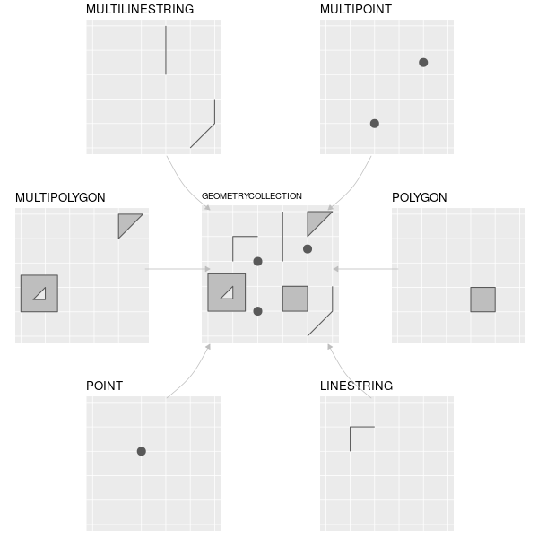
sf. Taken from Geocomputation with R.
sf is the main package we focus on in this section. Plus, we take a look at three packages for spatial data visualisation: ggplot2 (Wickham et al. 2024), tmap (Tennekes 2023), and mapview (Appelhans et al. 2022).
We can load them as:
library(sf)       # vector spatial data classes and functions
library(ggplot2)  # non-spatial and spatial plotting
library(tmap)     # noninteractive and interactive maps
library(mapview)  # quick interactive maps
2.1 Read data into R
Reading data into R can be done from a local file or a remote file. If you downloaded the workshop repository, you will find the data in the data directory. But, we can also fetch the data from GitHub directly, without the need to download it.
rivers = read_sf(
  "https://github.com/loreabad6/egu24-sc-R4geosciences/raw/main/data/nz-river-centrelines-topo-1500k.gpkg"
)
As you may have guessed from the object name, this is a river centreline dataset in New Zealand (Topo, 1:500k). This data is from Land Information New Zealand
We can now print the data to see how it looks like.
riversSimple feature collection with 7894 features and 0 fields
Geometry type: MULTILINESTRING
Dimension: XY
Bounding box: xmin: 1090841 ymin: 4753217 xmax: 2085682 ymax: 6190544
Projected CRS: NZGD2000 / New Zealand Transverse Mercator 2000
# A tibble: 7,894 × 1
geom
<MULTILINESTRING [m]>
1 ((1188893 4876720, 1188961 4876789, 1189209 4876888, 1189352 4877037, 118941…
2 ((1212357 4985134, 1212190 4985017, 1212190 4984899, 1212240 4984833, 121222…
3 ((1793234 5835222, 1793051 5835188, 1793001 5835221, 1792804 5835245))
4 ((1237766 4958688, 1237833 4958555, 1237861 4958499, 1237950 4958321, 123818…
5 ((1479132 5112613, 1479112 5112458, 1479143 5112127, 1479307 5111749, 147945…
6 ((1331799 4889014, 1331743 4889153, 1331644 4889637, 1331644 4889652, 133164…
7 ((1421067 5030500, 1421156 5030431, 1421280 5030411, 1421412 5030354, 142154…
8 ((1137668 4888410, 1137186 4888320, 1136813 4888447, 1136732 4888437, 113655…
9 ((1460473 5142519, 1460661 5141978, 1460657 5141736, 1460724 5141519, 146086…
10 ((1473259 5181908, 1473317 5181722, 1473317 5181472, 1473417 5181388, 147353…
# ℹ 7,884 more rowsA sf object shows each observation in a row and each attribute in a column. The object header includes relevant spatial information about the object, like the number of rows and columns, the geometry type, dimensions, bounding box and the CRS. Our rivers object has only one column, the geometry column.
You can dive deeper into sf objects and simple features in the package documentation here.
2.2 Projections and transformations
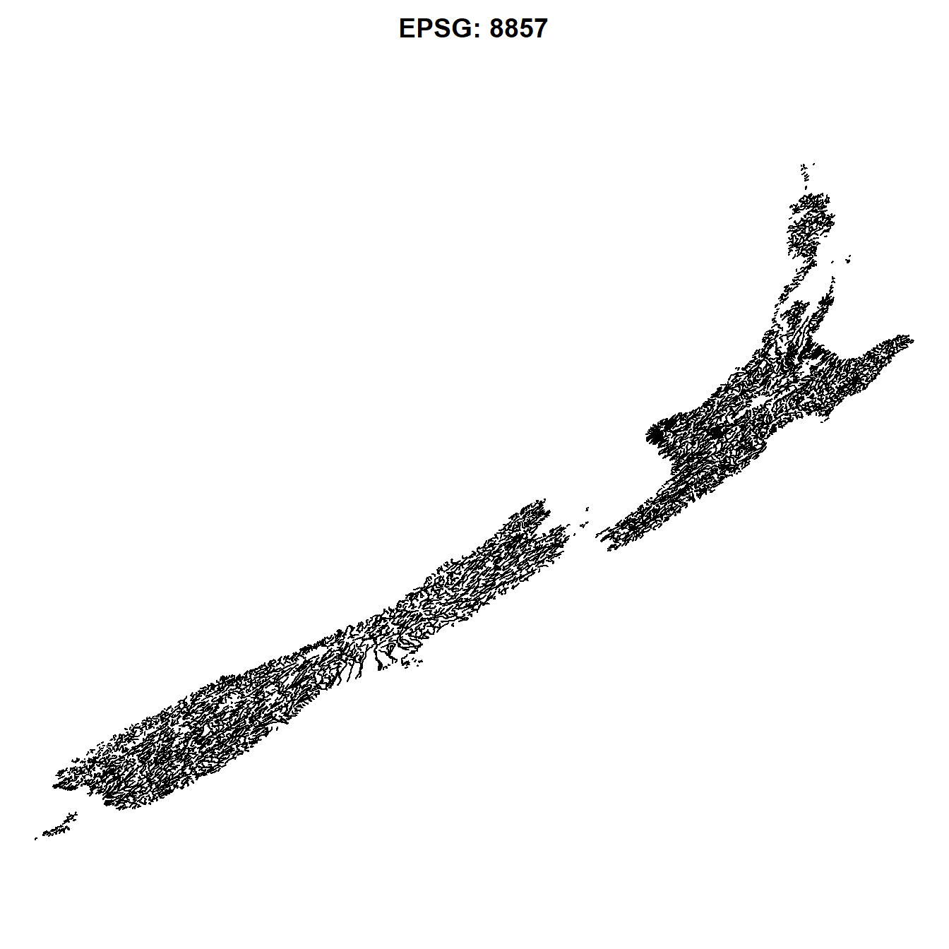
Geographical data has a Coordinate Reference System (CRS) that allows its location on the Earth surface. We can see the CRS of our rivers object using sf::st_crs() and we can easily transform the CRS using sf::st_transform().
st_crs(rivers)Coordinate Reference System:
User input: NZGD2000 / New Zealand Transverse Mercator 2000
wkt:
PROJCRS["NZGD2000 / New Zealand Transverse Mercator 2000",
BASEGEOGCRS["NZGD2000",
DATUM["New Zealand Geodetic Datum 2000",
ELLIPSOID["GRS 1980",6378137,298.257222101,
LENGTHUNIT["metre",1]]],
PRIMEM["Greenwich",0,
ANGLEUNIT["degree",0.0174532925199433]],
ID["EPSG",4167]],
CONVERSION["New Zealand Transverse Mercator 2000",
METHOD["Transverse Mercator",
ID["EPSG",9807]],
PARAMETER["Latitude of natural origin",0,
ANGLEUNIT["degree",0.0174532925199433],
ID["EPSG",8801]],
PARAMETER["Longitude of natural origin",173,
ANGLEUNIT["degree",0.0174532925199433],
ID["EPSG",8802]],
PARAMETER["Scale factor at natural origin",0.9996,
SCALEUNIT["unity",1],
ID["EPSG",8805]],
PARAMETER["False easting",1600000,
LENGTHUNIT["metre",1],
ID["EPSG",8806]],
PARAMETER["False northing",10000000,
LENGTHUNIT["metre",1],
ID["EPSG",8807]]],
CS[Cartesian,2],
AXIS["northing (N)",north,
ORDER[1],
LENGTHUNIT["metre",1]],
AXIS["easting (E)",east,
ORDER[2],
LENGTHUNIT["metre",1]],
USAGE[
SCOPE["Engineering survey, topographic mapping."],
AREA["New Zealand - North Island, South Island, Stewart Island - onshore."],
BBOX[-47.33,166.37,-34.1,178.63]],
ID["EPSG",2193]]st_transform(rivers, "EPSG:8857")Simple feature collection with 7894 features and 0 fields
Geometry type: MULTILINESTRING
Dimension: XY
Bounding box: xmin: 13541120 ymin: -5703283 xmax: 15383260 ymax: -4285790
Projected CRS: WGS 84 / Equal Earth Greenwich
# A tibble: 7,894 × 1
geom
* <MULTILINESTRING [m]>
1 ((13666283 -5587607, 13666417 -5587547, 13666759 -5587469, 13667045 -5587338…
2 ((13793866 -5486106, 13793590 -5486208, 13793478 -5486320, 13793464 -5486386…
3 ((15102339 -4651778, 15102131 -4651817, 15102106 -4651784, 15101929 -4651764…
4 ((13793768 -5512762, 13793707 -5512892, 13793682 -5512947, 13793600 -5513121…
5 ((14180046 -5373670, 14179883 -5373819, 14179614 -5374140, 14179436 -5374509…
6 ((13821294 -5583471, 13821371 -5583337, 13821736 -5582874, 13821750 -5582860…
7 ((14045490 -5451552, 14045517 -5451621, 14045623 -5451643, 14045704 -5451702…
8 ((13627195 -5573120, 13626635 -5573172, 13626393 -5573025, 13626304 -5573028…
9 ((14188313 -5344329, 14188013 -5344858, 14187789 -5345092, 14187659 -5345304…
10 ((14236840 -5306286, 14236731 -5306469, 14236506 -5306712, 14236532 -5306795…
# ℹ 7,884 more rowsCode
par(mar = c(0,0,2,0))
rivers |> plot(main = "EPSG: 2193")
# WGS 84 / Equal Earth Greenwich
st_transform(rivers, 8857) |> plot(main = "EPSG: 8857")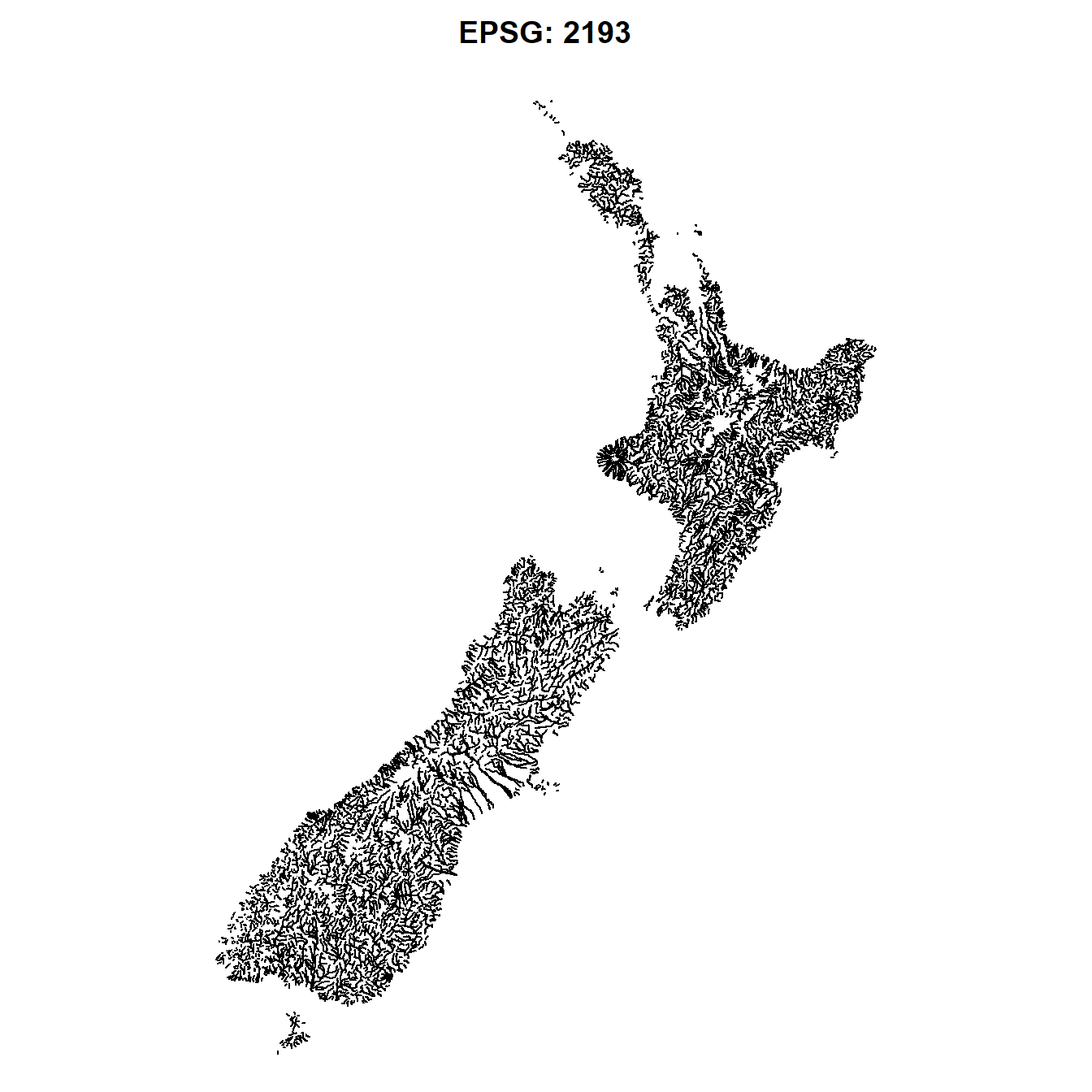
![]() Section in Spatial Data Science (Pebesma and Bivand 2023a)
Section in Spatial Data Science (Pebesma and Bivand 2023a)
![]() Section in Geocomputation with R (Lovelace, Nowosad, and Muenchow 2019).
Section in Geocomputation with R (Lovelace, Nowosad, and Muenchow 2019).
2.3 Geometrical operations
Basic geometric operations such as calculating the length or area of a geometry are supported. Let’s create a new column in our data with the river length as:
rivers["length"] = st_length(rivers)
rivers
Simple feature collection with 7894 features and 1 field
Geometry type: MULTILINESTRING
Dimension: XY
Bounding box: xmin: 1090841 ymin: 4753217 xmax: 2085682 ymax: 6190544
Projected CRS: NZGD2000 / New Zealand Transverse Mercator 2000
# A tibble: 7,894 × 2
geom length
<MULTILINESTRING [m]> [m]
1 ((1188893 4876720, 1188961 4876789, 1189209 4876888, 1189352 4877037,… 73029.
2 ((1212357 4985134, 1212190 4985017, 1212190 4984899, 1212240 4984833,… 45755.
3 ((1793234 5835222, 1793051 5835188, 1793001 5835221, 1792804 5835245)) 445.
4 ((1237766 4958688, 1237833 4958555, 1237861 4958499, 1237950 4958321,… 32311.
5 ((1479132 5112613, 1479112 5112458, 1479143 5112127, 1479307 5111749,… 1391.
6 ((1331799 4889014, 1331743 4889153, 1331644 4889637, 1331644 4889652,… 61151.
7 ((1421067 5030500, 1421156 5030431, 1421280 5030411, 1421412 5030354,… 36612.
8 ((1137668 4888410, 1137186 4888320, 1136813 4888447, 1136732 4888437,… 1622.
9 ((1460473 5142519, 1460661 5141978, 1460657 5141736, 1460724 5141519,… 2582.
10 ((1473259 5181908, 1473317 5181722, 1473317 5181472, 1473417 5181388,… 53171.
# ℹ 7,884 more rowsTo show other operations, we load another dataset. This are administrative areas in New Zealand. The data comes from the spData package, which is a data package that has some example datasets.
data("nz", package = "spData")
nz
Simple feature collection with 16 features and 6 fields
Geometry type: MULTIPOLYGON
Dimension: XY
Bounding box: xmin: 1090144 ymin: 4748537 xmax: 2089533 ymax: 6191874
Projected CRS: NZGD2000 / New Zealand Transverse Mercator 2000
First 10 features:
Name Island Land_area Population Median_income Sex_ratio
1 Northland North 12500.561 175500 23400 0.9424532
2 Auckland North 4941.573 1657200 29600 0.9442858
3 Waikato North 23900.036 460100 27900 0.9520500
4 Bay of Plenty North 12071.145 299900 26200 0.9280391
5 Gisborne North 8385.827 48500 24400 0.9349734
6 Hawke's Bay North 14137.524 164000 26100 0.9238375
7 Taranaki North 7254.480 118000 29100 0.9569363
8 Manawatu-Wanganui North 22220.608 234500 25000 0.9387734
9 Wellington North 8048.553 513900 32700 0.9335524
10 West Coast South 23245.456 32400 26900 1.0139072
geom
1 MULTIPOLYGON (((1745493 600...
2 MULTIPOLYGON (((1803822 590...
3 MULTIPOLYGON (((1860345 585...
4 MULTIPOLYGON (((2049387 583...
5 MULTIPOLYGON (((2024489 567...
6 MULTIPOLYGON (((2024489 567...
7 MULTIPOLYGON (((1740438 571...
8 MULTIPOLYGON (((1866732 566...
9 MULTIPOLYGON (((1881590 548...
10 MULTIPOLYGON (((1557042 531...summary(nz) Name Island Land_area Population
Length:16 Length:16 Min. : 422.2 Min. : 32400
Class :character Class :character 1st Qu.: 8301.5 1st Qu.: 51325
Mode :character Mode :character Median :12285.9 Median : 169750
Mean :16505.5 Mean : 299200
3rd Qu.:23409.1 3rd Qu.: 339950
Max. :44504.5 Max. :1657200
Median_income Sex_ratio geom
Min. :23400 Min. :0.9238 MULTIPOLYGON :16
1st Qu.:26000 1st Qu.:0.9346 epsg:2193 : 0
Median :27050 Median :0.9477 +proj=tmer...: 0
Mean :27375 Mean :0.9518
3rd Qu.:29200 3rd Qu.:0.9613
Max. :32700 Max. :1.0139 We proceed to filter our data to one of NZ regions, Gisborne.
(gisborne = nz[nz$Name == "Gisborne", ])Simple feature collection with 1 feature and 6 fields
Geometry type: MULTIPOLYGON
Dimension: XY
Bounding box: xmin: 1959096 ymin: 5674920 xmax: 2089533 ymax: 5833212
Projected CRS: NZGD2000 / New Zealand Transverse Mercator 2000
Name Island Land_area Population Median_income Sex_ratio
5 Gisborne North 8385.827 48500 24400 0.9349734
geom
5 MULTIPOLYGON (((2024489 567...plot(nz$geom)
plot(gisborne$geom)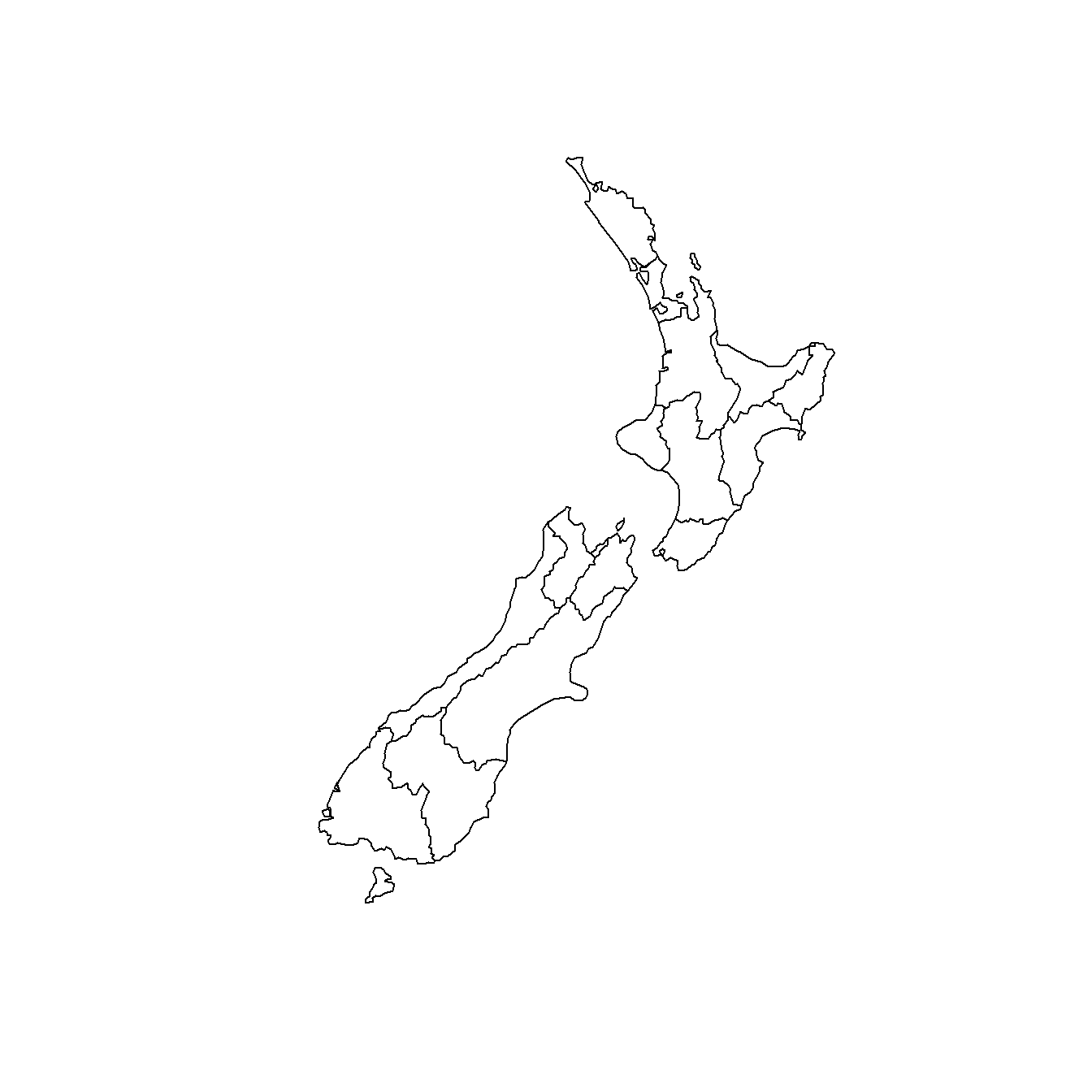
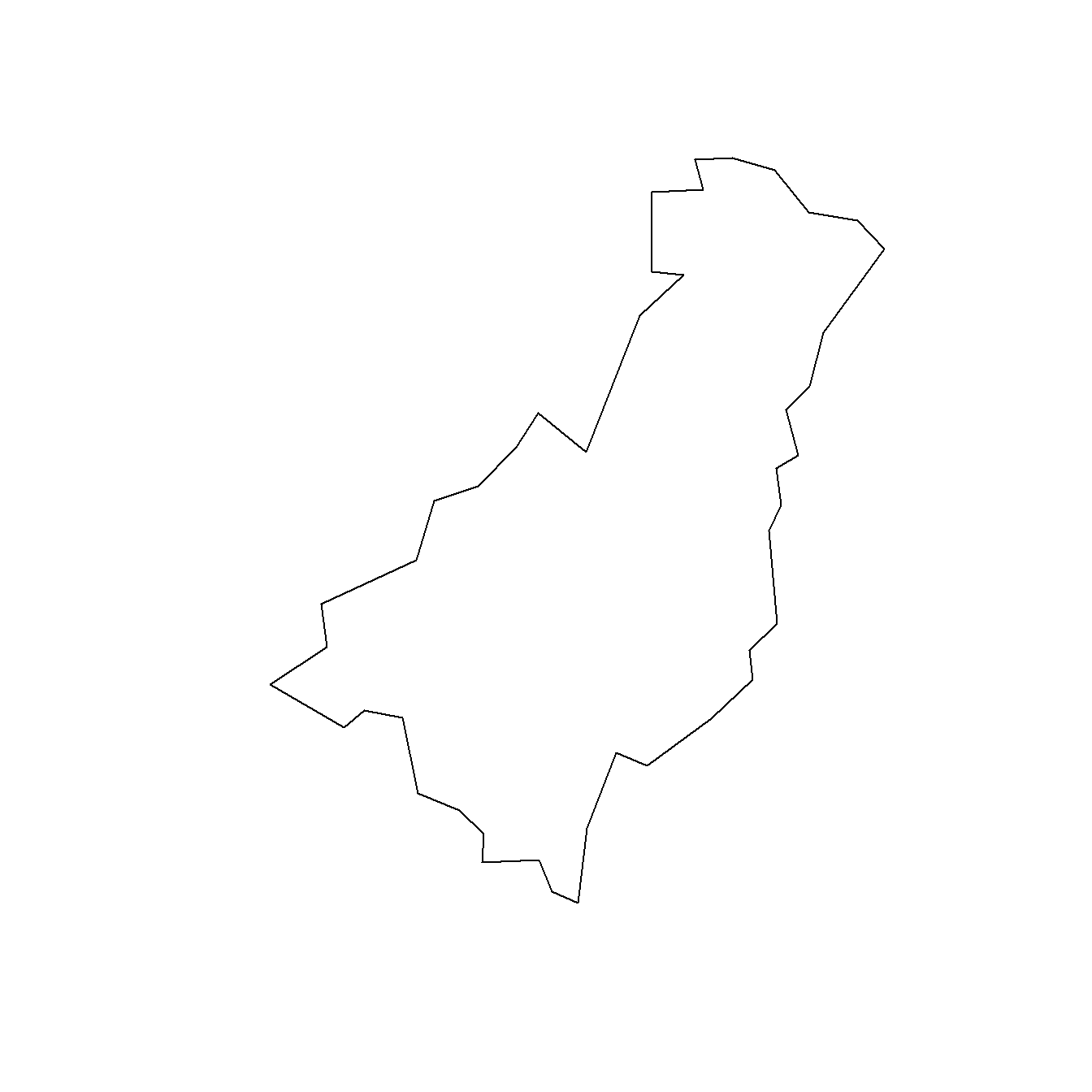
Now, we can do operations like spatial filters and operations. Let’s try filter the river data for the Gisborne region.

rivers |> st_intersection(gisborne)Error in geos_op2_geom("intersection", x, y, ...): st_crs(x) == st_crs(y) is not TRUEThat gave us an error since the data is not projected in to the same CRS.
gisborne = st_transform(gisborne, st_crs(rivers))Let’s try that again.
rivers |> st_intersection(gisborne)Warning: attribute variables are assumed to be spatially constant throughout
all geometriesSimple feature collection with 286 features and 7 fields
Geometry type: GEOMETRY
Dimension: XY
Bounding box: xmin: 1964161 ymin: 5676307 xmax: 2085682 ymax: 5829474
Projected CRS: NZGD2000 / New Zealand Transverse Mercator 2000
# A tibble: 286 × 8
length Name Island Land_area Population Median_income Sex_ratio
* [m] <chr> <chr> <dbl> <dbl> <int> <dbl>
1 25580. Gisborne North 8386. 48500 24400 0.935
2 55146. Gisborne North 8386. 48500 24400 0.935
3 30760. Gisborne North 8386. 48500 24400 0.935
4 28458. Gisborne North 8386. 48500 24400 0.935
5 29961. Gisborne North 8386. 48500 24400 0.935
6 25386. Gisborne North 8386. 48500 24400 0.935
7 28251. Gisborne North 8386. 48500 24400 0.935
8 28476. Gisborne North 8386. 48500 24400 0.935
9 29663. Gisborne North 8386. 48500 24400 0.935
10 9291. Gisborne North 8386. 48500 24400 0.935
# ℹ 276 more rows
# ℹ 1 more variable: geom <LINESTRING [m]>We just intersected the river data with the data in the gisborne object. What we are doing is an inner spatial join, where only those river linestrings that intersect the gisborne object stay. Another way to do this is:
rivers |> st_join(gisborne, left = FALSE, join = st_intersects)Simple feature collection with 286 features and 7 fields
Geometry type: MULTILINESTRING
Dimension: XY
Bounding box: xmin: 1964161 ymin: 5665081 xmax: 2085682 ymax: 5830551
Projected CRS: NZGD2000 / New Zealand Transverse Mercator 2000
# A tibble: 286 × 8
geom length Name Island Land_area Population
* <MULTILINESTRING [m]> [m] <chr> <chr> <dbl> <dbl>
1 ((2020380 5682629, 2020497 5682630,… 25580. Gisb… North 8386. 48500
2 ((2047236 5739047, 2047119 5738963,… 55146. Gisb… North 8386. 48500
3 ((1992989 5756684, 1992939 5756835,… 30760. Gisb… North 8386. 48500
4 ((2009450 5761922, 2009383 5761988,… 28458. Gisb… North 8386. 48500
5 ((2059935 5763492, 2059842 5763462,… 29961. Gisb… North 8386. 48500
6 ((2027788 5774462, 2027789 5774211,… 25386. Gisb… North 8386. 48500
7 ((2035023 5793818, 2035107 5793618,… 28251. Gisb… North 8386. 48500
8 ((2064446 5774410, 2064479 5774661,… 28476. Gisb… North 8386. 48500
9 ((2083085 5804913, 2082742 5805001,… 29663. Gisb… North 8386. 48500
10 ((1998917 5702907, 1998927 5702908,… 9291. Gisb… North 8386. 48500
# ℹ 276 more rows
# ℹ 2 more variables: Median_income <int>, Sex_ratio <dbl>The join parameter allows you to add any other type of DE-9IM relation, including your own. So, if we want to get those river linestrings that are within the gisborne object we would use sf::st_within().
rivers |> st_join(gisborne, left = FALSE, join = st_within)Simple feature collection with 248 features and 7 fields
Geometry type: MULTILINESTRING
Dimension: XY
Bounding box: xmin: 1967989 ymin: 5687240 xmax: 2085682 ymax: 5829458
Projected CRS: NZGD2000 / New Zealand Transverse Mercator 2000
# A tibble: 248 × 8
geom length Name Island Land_area Population
* <MULTILINESTRING [m]> [m] <chr> <chr> <dbl> <dbl>
1 ((2047236 5739047, 2047119 5738963,… 55146. Gisb… North 8386. 48500
2 ((2009450 5761922, 2009383 5761988,… 28458. Gisb… North 8386. 48500
3 ((2059935 5763492, 2059842 5763462,… 29961. Gisb… North 8386. 48500
4 ((2027788 5774462, 2027789 5774211,… 25386. Gisb… North 8386. 48500
5 ((2064446 5774410, 2064479 5774661,… 28476. Gisb… North 8386. 48500
6 ((1998917 5702907, 1998927 5702908,… 9291. Gisb… North 8386. 48500
7 ((2001680 5712195, 2001746 5712112,… 8166. Gisb… North 8386. 48500
8 ((2068319 5787066, 2067617 5787365,… 6851. Gisb… North 8386. 48500
9 ((2058857 5789186, 2058757 5789287,… 8277. Gisb… North 8386. 48500
10 ((2070487 5798783, 2070335 5799153,… 8971. Gisb… North 8386. 48500
# ℹ 238 more rows
# ℹ 2 more variables: Median_income <int>, Sex_ratio <dbl>If we don’t want to do a join, that is if we don’t want to bring in the columns from the second dataset, we can use sf::st_filter(). We can also specify the DE-9IM relation here with the parameter .predicate
rivers |> st_filter(gisborne, .predicate = st_within)Simple feature collection with 248 features and 1 field
Geometry type: MULTILINESTRING
Dimension: XY
Bounding box: xmin: 1967989 ymin: 5687240 xmax: 2085682 ymax: 5829458
Projected CRS: NZGD2000 / New Zealand Transverse Mercator 2000
# A tibble: 248 × 2
geom length
* <MULTILINESTRING [m]> [m]
1 ((2047236 5739047, 2047119 5738963, 2047119 5738846, 2047002 5738779,… 55146.
2 ((2009450 5761922, 2009383 5761988, 2009365 5762322, 2009332 5762372,… 28458.
3 ((2059935 5763492, 2059842 5763462, 2059015 5763608, 2059005 5763649,… 29961.
4 ((2027788 5774462, 2027789 5774211, 2027839 5774111, 2027956 5773978,… 25386.
5 ((2064446 5774410, 2064479 5774661, 2064680 5774745, 2064713 5774812,… 28476.
6 ((1998917 5702907, 1998927 5702908, 1999151 5702924, 1999234 5702834,… 9291.
7 ((2001680 5712195, 2001746 5712112, 2001747 5711995, 2001663 5711761,… 8166.
8 ((2068319 5787066, 2067617 5787365, 2067366 5787398, 2067249 5787482,… 6851.
9 ((2058857 5789186, 2058757 5789287, 2058590 5789253, 2058556 5789286,… 8277.
10 ((2070487 5798783, 2070335 5799153, 2070277 5799363, 2070312 5799653,… 8971.
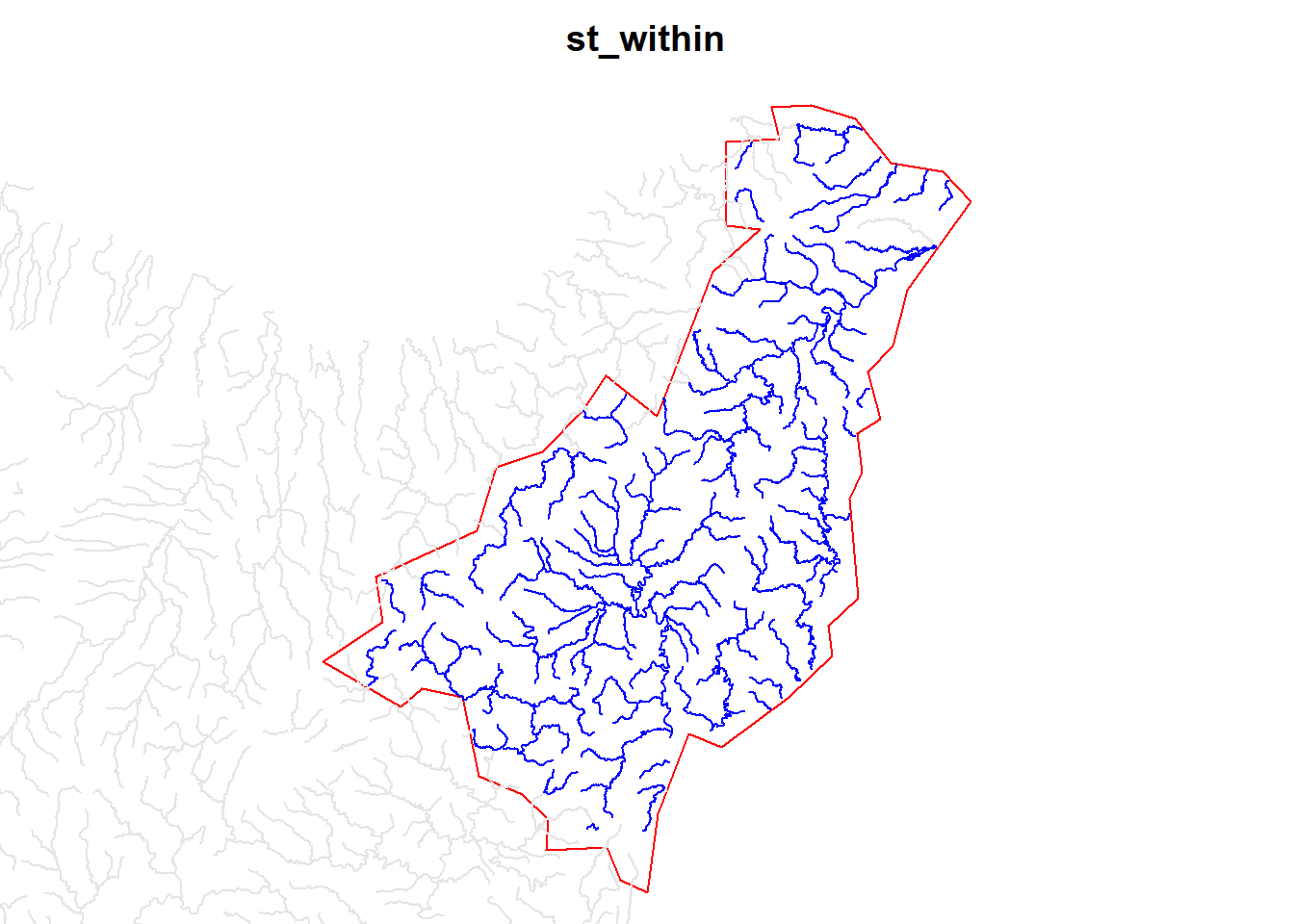
# ℹ 238 more rowsThis is a small plot of the difference between st_intersects and st_within.
Code
par(mar = c(0,0,2,0))
int = rivers |> st_filter(gisborne, .predicate = st_intersects)
with = rivers |> st_filter(gisborne, .predicate = st_within)
plot(gisborne$geom, border = "red", col = NA, main = "st_intersects")
plot(rivers$geom, col = "grey90", alpha = 0.5, add = TRUE)
plot(int$geom, col = "blue", add = TRUE)
plot(gisborne$geom, border = "red", col = NA, main = "st_within")
plot(rivers$geom, col = "grey90", alpha = 0.5, add = TRUE)
plot(with$geom, col = "blue", add = TRUE)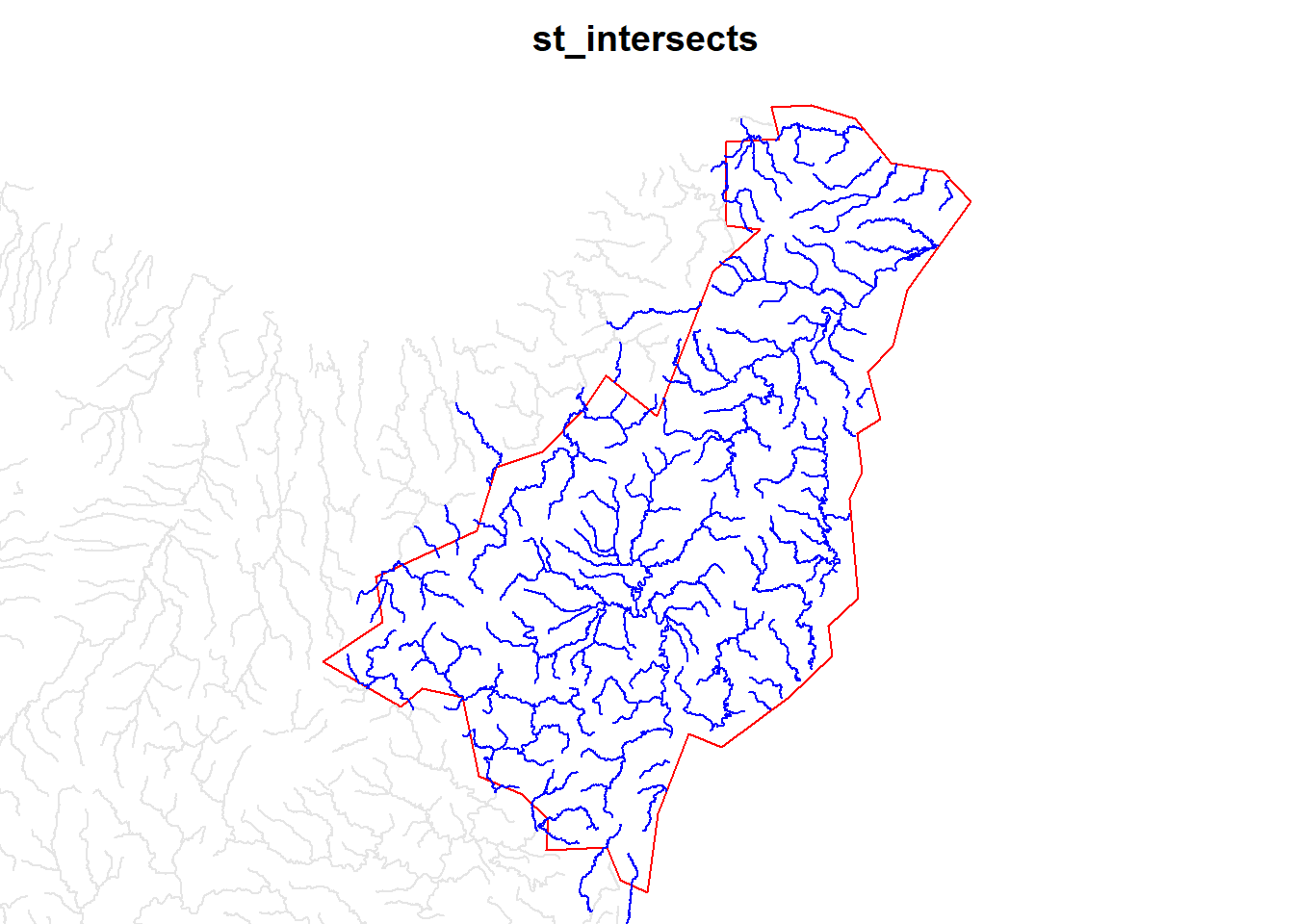
![]() Section in Spatial Data Science (Pebesma and Bivand 2023a)
Section in Spatial Data Science (Pebesma and Bivand 2023a)
![]() Section in Geocomputation with R (Lovelace, Nowosad, and Muenchow 2019).
Section in Geocomputation with R (Lovelace, Nowosad, and Muenchow 2019).
2.4 Plot spatial data
Some plots have already been shown in the sections above, but let’s look at this with more attention now.
2.4.1 Base R
sf has a base plot method, which plots in small subsets the different columns of the geospatial dataset.
plot(nz)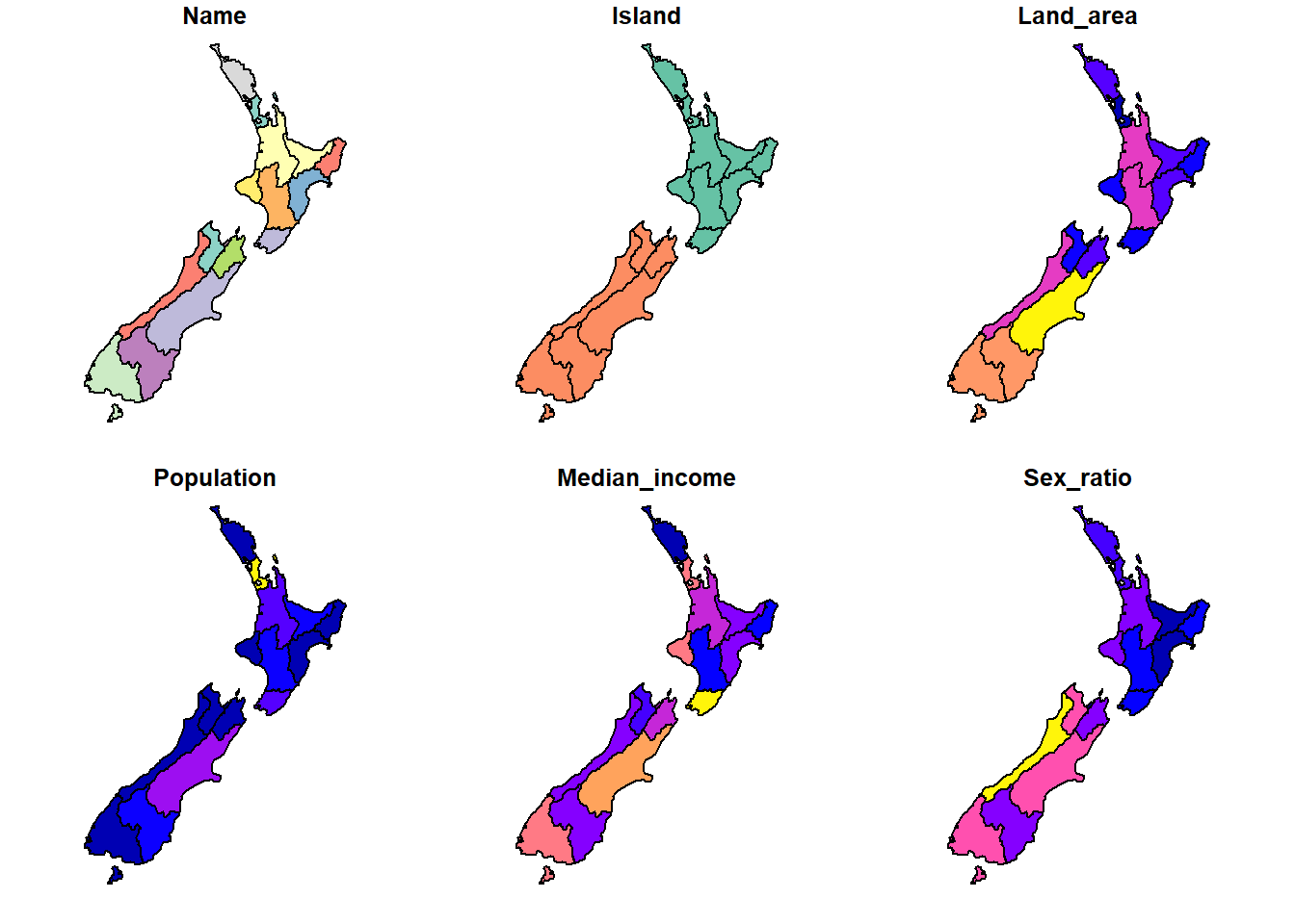
This is a great way to get a quick glance at how the data look likes.
2.4.2 ggplot2
There is a ggplot method for sf objects, where we use the ggplot2::geom_sf() function to plot the sf layer. As normal, we can call color and fill options with the data columns. There is no need to specify any x/y coordinates since the geometry is recognised automatically.
ggplot(nz) +
  geom_sf(aes(fill = Population))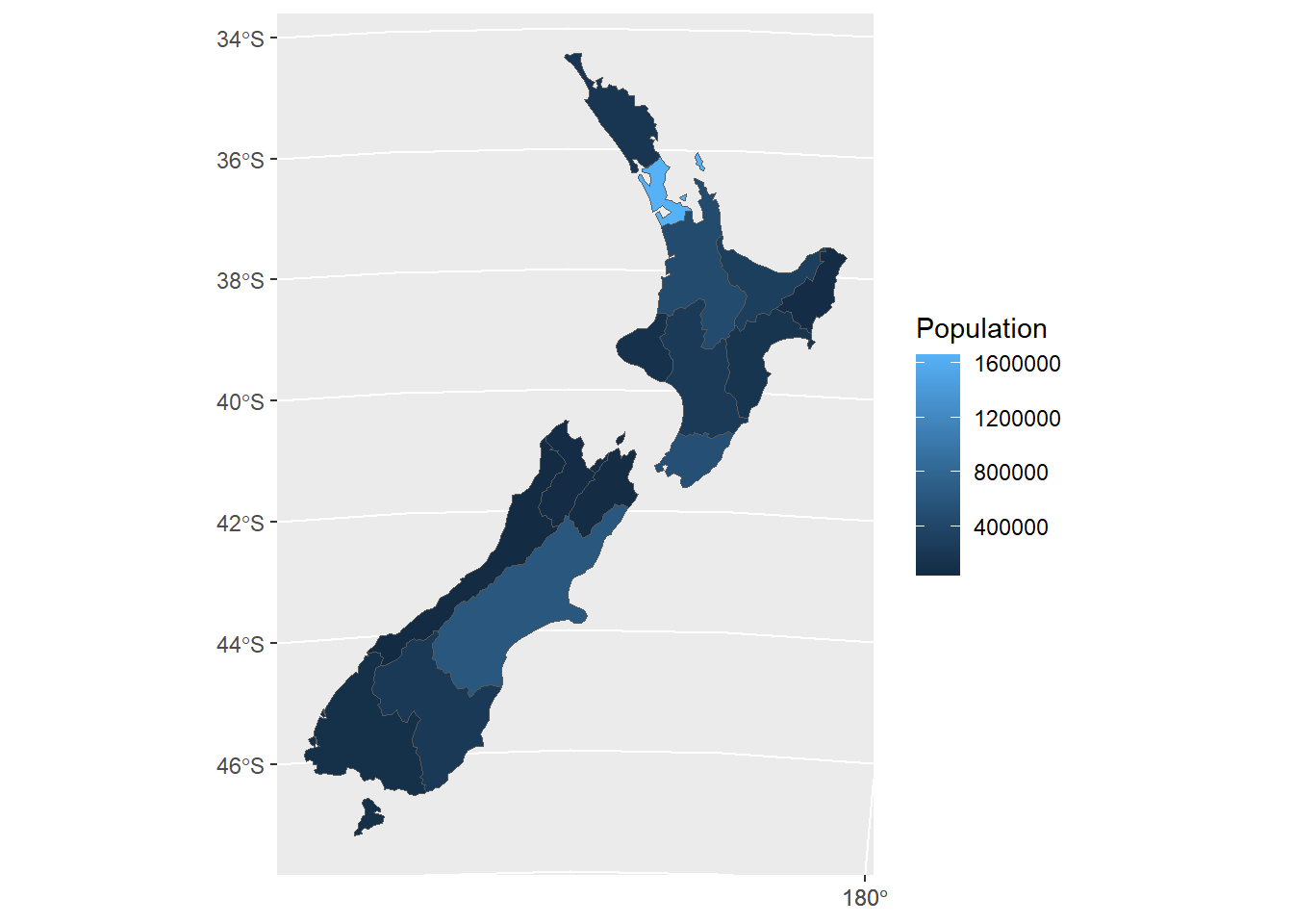
A great companion for making maps with {ggplot2} is {ggspatial}!
2.4.3 tmap v.4
tmap is another option for plotting spatial features. The package is on its way to a new version, with several breaking changes. Therefore, in this repository we have installed version 4 (the newer version) to showcase its usage.
tm_shape(nz) +
  tm_fill("Name") +
  tm_shape(rivers) +
  tm_lines(col = "white", lwd = 0.7) +
  tm_scalebar()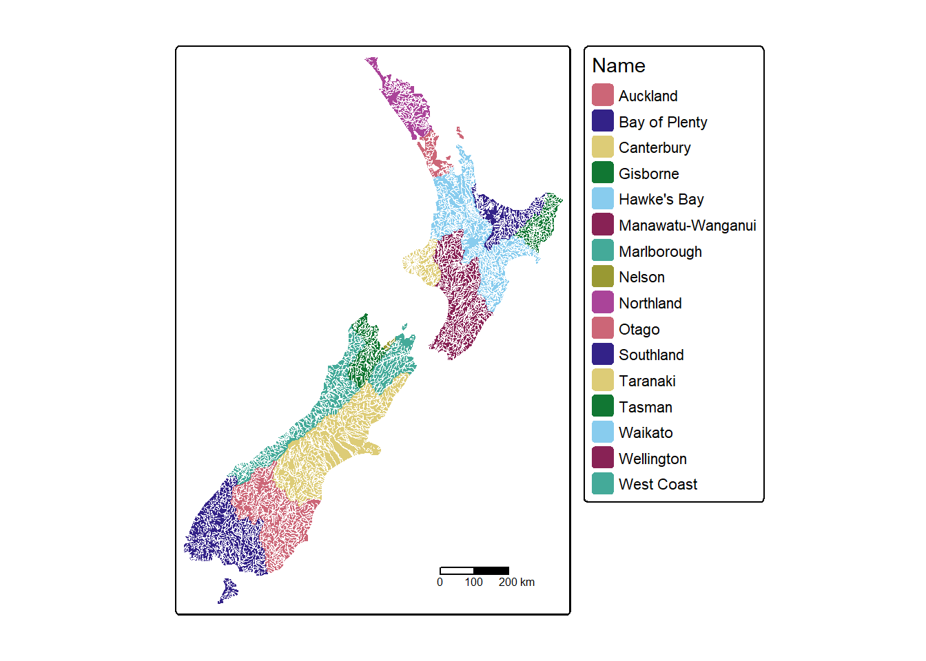
2.4.4 mapview
Finally, R has packages for interactive maps as well. While tmap can display some nice interactive maps, another option is mapview.
mapview(nz, zcol = "Median_income")You can find links to other R packages and resources for data visualisation here.