4 GIS: in-house and bridges
In this session you should learn:
Save the code you work on today, we will use it next week. Most importantly, try to automate the workflow using a function!
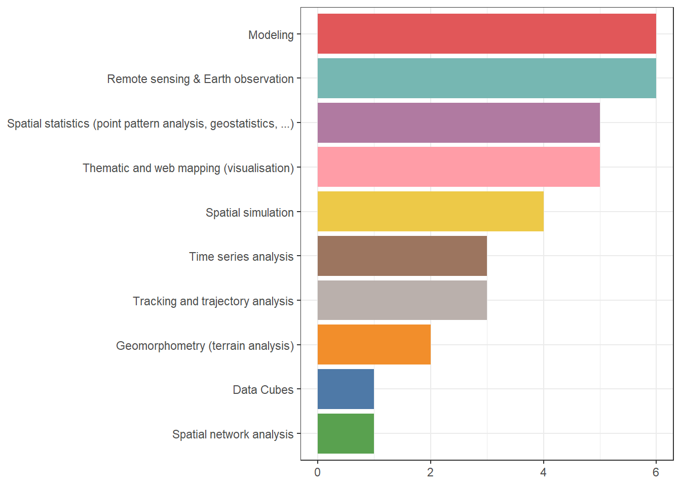
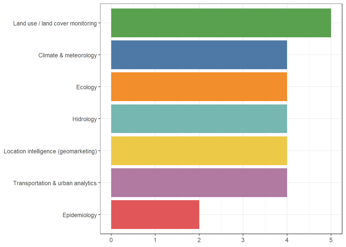
Thank you for replying to the poll last week! Here are the results:
4.1 Dedicated R packages
There are several packages in R that are specialised in particular spatial analysis methods so that you can do any analysis in R directly without resorting to external software. This is by all means not an exhaustive list of all the spatial capabilities in R, but just a sample to get you started.
4.1.1 Earth observation analytics and remote sensing
Remote sensing and Earth observation has had a big boost recently, especially since the ability to work with data out-of-memory1. Several workflows have become available to work with EO data within R to harness the statistical and visualisation capabilities of the programming language. Further, packages that allow retreival of EO data from cloud services are also available.
I. Statistical modelling and machine learning
Several packages are available to work with raster data as we saw last session, including {stars} and {terra}. One of the main use cases of raster data is to perform machine learning or statistical modelling.
Resources available:
II. Cloud data and on-demand data cubes
With the advent of common standards and specifications such as the Spatio Temporal Asset Catalog (STAC), accessing data from the cloud has become much easier. Once data can be accessed in an standardised way, working with on-demand data cubes locally becomes a much easier process.
The package {rstac} provides the workforce to fetch STAC data. This package is the basis for other packages workflows to download data, to create data cubes, or to do it all at once.
![]() Here you will find the package documentation.
Here you will find the package documentation.
Another interesting package is {rsi}, which stands for remote sensing indices. The package basically obtains data using {rstac} but also connects to the Awesome Spectral Indices catalogue to fetch standardised ways to compute popular spectral indices on your data.
![]() Resources for
Resources for {rsi}:
- Package documentation
- Blogpost: An overview of the rsi R package for retrieving satellite imagery and calculating spectral indices by Rydzik (2024)
Finally, the creation of on-demand data cubes is taken care of in R using the {gdalcubes} package. With this package you can create data cubes from cloud resources or local files, apply data cube operations (apply functions over dimensions, filtering, computing statistics with reductions), extract time series, create training data for machine learning.
![]() Resources for
Resources for {gdalcubes}:
III. All-in-one solution
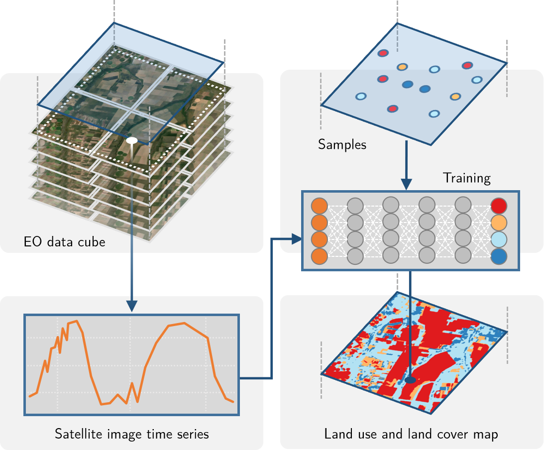
To concentrate all the efforts of fetching data from the cloud, creating on-demand data cubes, and performing statistical modelling or applying machine learning algorithms to the data, the {sits} package was created. It build upon the packages shown above and it can be seen as an all-in-one solution that simplifies the usage of satellite imagery time series. The main focus is of course on time series analysis, therefore taking the time component into account for the modelling.
A typical workflow in {sits} would look like this:
 Resources for
 {sits}:
4.1.2 Spatial statistics
R is well know for its statistical capabilities, and spatial statistics is no exception. Several packages allow for full statistical analysis workflows like:
- point pattern analysis using
{spatstat}- Package resources
- Chapter: Point Pattern Analysis in E. Pebesma & Bivand (2023)
- interpolation and geostatistics with
{gstat}- Chapter: Spatial Interpolation in E. Pebesma & Bivand (2023)
- Package reference
- autocorrelation and spatial dependence with
{spdep}and{rgeoda}- Chapter: Proximity and Areal Data in E. Pebesma & Bivand (2023)
- Chapter: Measures of Spatial Autocorrelation in E. Pebesma & Bivand (2023)
{rgeoda}package documentation{spdep}package documentation- Tidyverse friendly package
{sfdep}documentation
- … many others (see further reading)
4.1.3 Spatial network analysis
Working with spatial networks in R used to be a bit of a difficult taks before the package {sfnetworks} arrived. The aim of the package is to bridge between {sf} and {tidygraph} a tidy wrapper of the C++ {igraph} library which is used very often for network analysis.
With {sfnetworks} you can perform several tasks such as:
- creating networks from points and lines
- network cleaning
- finding shortest paths
- route optimisation
- closest facility analysis
- creating catchment areas
- zoning networks based on their connectivity
- …
It started as an assignment for an R course in an effort to find an open source solution to the ArcGIS network analysis capabilities and is now downloaded over 2 thousand times a month!
![]() I recommend you to work with the development version (here are the docs).
I recommend you to work with the development version (here are the docs).
4.2 Bridges to external software
Of course, you can also connect to external GIS software to perform operations in R. Why would you want to do that? One good reason is to automate your workflows. Instead of following a click, click, click sequence, you can have your process in a coded written form that allows you to remember what you did as it is written and documented, but also perform the same process over and over via automation.
4.2.1 QGIS
One of the best bridges to GIS with R out there is the {qgisprocess} package, which wraps around the “qgis process” command line. There is also a {qgis} package with the same idea but does a function per algorithm. It does not only give you access to native QGIS processing tools but also to any other add-on you have made available via your QGIS installation including plug-ins. That means, GRASS GIS, GDAL, SAGA are fully available to you via inside R with one package!
 Resources to bridge with QGIS
{qgisprocess}package documentation{qgis}package documentation- Section in Bridges to GIS software in Lovelace et al. (2019)
- Presentation at UseR! 2024 by Floris Vanderhaeghe for more info on
{qgis}and{qgisprocess}
Naturally, for this to work, you will need a QGIS installation. The package will try to find your installation automatically on your first run. However, you can also pass a custom path if you have multiple installations.
Depending on your QGIS configuration, you will have access to different providers. You can look at what is available to you with qgis_providers().
4.2.2 SAGA GIS
You also have individual bridges to GIS software naturally. If you are interested in geomorphology and hydrology, you might be very familiar with SAGA GIS. You can access SAGA algorithms via QGIS, but if you don’t have that linked or if you rather use a package with less dependencies, then {Rsagacmd} is for you. There is also the {RSAGA} package, however, this does not have so good documentation, and its development seems a bit paused.
![]() Resources for SAGA GIS bridges with R
Resources for SAGA GIS bridges with R
- Package documentation for
{Rsagacmd} - Section in Bridges to GIS software in Lovelace et al. (2019)
- The GitHub repository of the
{RSAGA}package - A package I built to automise my workflows based on
{RSAGA}
Again, you will need to have a SAGA GIS installation or point the package to the installation path of the SAGA GIS version you would like to use.
4.2.3 GRASS GIS
Does anyone know what GRASS2 stands for?
GRASS GIS has been around since the 80s and is one of the most powerful GIS out there. It has been ahead of its time for so long and it keeps up-to-date with current GIS trends. Its community of developers and users is also thriving, even having annual workshops that allow the further development of the tools supported.
It is a core part of the OSGeo suite of sofware, available in loads of languages, has really good cloud-support and as one of the core members, Vero Andreo always likes to say: it rocks!
 Resources to work with GRASS GIS
{rgrass}package documentation- Tutorial: Get started with GRASS & R: the rgrass package by Andreo (2024)
- Presentation at UseR! 2024 by Vero Andreo (core member of GRASS GIS)
- Section in Bridges to GIS software in Lovelace et al. (2019)
- Modernizing the R-GRASS interface: confronting barn-raised OSGeo libraries and the evolving R.*spatial package ecosystem by R. Bivand (2022)
Naturally, you will need an installation of GRASS to be able to run the algorithms with this package.
4.2.4 Google Earth Engine (GEE)
Bindings to GEE are available via the {rgee} package. The efforts towards this connection were driven by a former student here at PLUS! It does not only have now the connection to GEE but also functions that build on top of it and a book with good documentation.


This bridge of course requires you to have a Google Earth Engine account that will allow you to authenticate. The documentation of the package has all the required steps to get started.
4.2.5 R-ArcGIS Bridge
ESRI has also made efforts to connect to open source software. You already know how to connect ArcGIS to Python, using the arcpy interface. For R, ESRI has created a bundle of packages that, when you have ArcGIS Pro and a valid license, you can use to run their geoprocessing tools.
![]() Here you can find the documentation to install and quick start with these packages.
Here you can find the documentation to install and quick start with these packages.
I will not support your use of proprietary software in this course, but if you are interested and even if you would like to use it in your project, feel free to do so.
4.3 Hands-on
4.4 Further reading:
- Models for spatial data section, chapters 10-15 (E. Pebesma & Bivand, 2023)
- Statistical learning chapter (Lovelace et al., 2019)
- Bridges to GIS software chapter (Lovelace et al., 2019)
- Remote sensing in R discussion on R-Spatial organization on GitHub